How do you design an RF amplifier using GaN transistors? Begin with a measurable RF specification, choose a GaN HEMT with an appropriate frequency and power range, establish a safe bias procedure, prove stability over a frequency range wider than the intended band, obtain source and load impedances for the target operating class, synthesize the matching networks, design the thermal and PCB structure, then validate small-signal and large-signal performance on calibrated hardware.
GaN offers high breakdown field, high power density, useful high-frequency gain, and the ability to operate at elevated drain voltage. Those advantages do not eliminate ordinary RF design constraints. A successful amplifier still depends on the device model, bias network, package reference planes, matching loss, harmonic terminations, stability, heat flow, and measurement discipline.
1. Define the amplifier specification
Do not select a transistor before defining the job. Record at least:
- Center frequency and operating bandwidth
- Continuous-wave, pulsed, or modulated waveform
- Required output power, gain, and gain flatness
- Drain efficiency or power-added efficiency target
- Linearity targets such as EVM, ACLR, IMD, or spectral mask
- Supply voltage and available driver power
- Permitted input and output return loss
- Expected antenna or load mismatch
- Baseplate temperature, pulse width, duty cycle, and cooling
- Size, cost, reliability, and qualification requirements
A narrowband continuous-wave industrial amplifier, a radar pulse amplifier, and a wideband communication transmitter can require different device peripheries, bias classes, matching networks, and thermal solutions. The communication application area provides useful system context, but the transistor must be selected from the actual RF load line.
2. Select the GaN transistor and model
Check the device’s frequency range, recommended drain voltage, output-power capability, gain, efficiency data, package style, thermal resistance, and ruggedness information. Review whether the available data represents pulsed or continuous-wave operation and whether the reference plane is at the package lead, fixture connector, or a de-embedded device plane.
Use the manufacturer’s nonlinear model when available. S-parameters describe linear behavior at a stated bias and power level. They are valuable for small-signal gain, input and output match, and stability analysis, but they do not by themselves predict compression, waveform clipping, current swing, trapping, self-heating, or harmonic behavior near rated power.
3. Choose an operating class and quiescent bias
Class A offers high linearity and conduction angle but poor efficiency. Class AB is common when the amplifier must balance gain, linearity, and efficiency. Class B or C can suit constant-envelope or nonlinear stages, while classes E, F, inverse F, and related harmonic-controlled modes pursue higher efficiency through waveform engineering.
Follow the device manufacturer’s bias procedure. Many depletion-mode RF GaN HEMTs require negative gate voltage before positive drain voltage is applied. A typical safe sequence is to establish the off-state gate bias, apply drain voltage, then adjust gate voltage until the specified quiescent drain current is reached. Power-down reverses the sequence. Exact voltages and currents must come from the chosen device documentation.
Gate leakage, temperature, active-bias stability, and bypass-capacitor current capability can move the operating point. A bias circuit must remain stable while presenting a high RF impedance at the transistor reference plane.
4. Analyze stability before matching for gain
Evaluate stability from frequencies well below the operating band to well above it. High-gain transistors can oscillate at low frequency through the bias network or at microwave frequencies through package, matching, or enclosure coupling.
Small-signal indicators such as Rollet’s K factor, the B1 measure, μ, and μ′ help identify unconditional or conditional stability under the modeled bias. Plot stability circles when needed. Repeat the analysis with component tolerances, bias-network models, package parasitics, and expected source and load impedances.
Stabilization may use a series gate resistor, shunt resistance, lossy feedback, frequency-selective networks, ferrite loading, or controlled matching. Avoid unnecessary output loss in a power amplifier. The network should provide margin without sacrificing required gain, noise, or output power.
5. Determine source and load impedances
For a small-signal amplifier, conjugate or gain-circle matching from S-parameters may be adequate. For a power amplifier, the optimum load at compression is generally not the small-signal conjugate of the output impedance.
Use simulated or measured load-pull data at the intended frequency, drain voltage, bias, drive level, and harmonic conditions. Select an impedance region that balances output power, efficiency, gain, and linearity rather than chasing one maximum point. Source-pull may improve gain or power delivery at the input.
Be explicit about impedance reference planes. Package parasitics and evaluation fixtures can rotate and transform the apparent impedance substantially. Moving a target from the intrinsic current-generator plane to the package lead or PCB plane requires the correct embedding network.
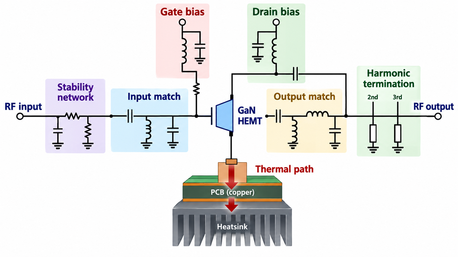
6. Synthesize the input and output matching networks
Transform 50 Ω to the selected source and load impedances using transmission lines, capacitors, inductors, transformers, or a combination. At microwave frequencies, microstrip and coplanar structures are distributed components, and pads, vias, launches, packages, and component bodies must be included in the electromagnetic model.
Start with an ideal network to understand the required transformation and loaded Q. Then replace ideal elements with realizable models. Include conductor loss, dielectric loss, component Q, self-resonance, current rating, and manufacturing tolerance. A very high transformation ratio can narrow bandwidth and magnify sensitivity.
The input match often balances return loss, transducer gain, stability, and driver loading. The output match must also carry high RF current and voltage without excessive loss or local heating.
7. Plan harmonic terminations
The impedance seen at the second and third harmonics can change drain-voltage and drain-current waveforms, efficiency, and peak device stress. Harmonic-controlled classes intentionally present open, short, or other target impedances at selected harmonics.
Even a conventional Class AB design should examine harmonic behavior. Bias chokes, radial stubs, package parasitics, connector transitions, and enclosure modes can create unintended resonances. Large-signal harmonic-balance simulation and EM co-simulation help expose these effects.
8. Design the gate and drain bias networks
Bias feeds must deliver DC while isolating the RF path. A quarter-wave line, high-impedance line, RF choke, radial stub, bypass-capacitor ladder, or combined network may be used depending on frequency and bandwidth.
- Place bypass capacitors in a hierarchy that remains effective from low frequency through the RF band.
- Model capacitor ESR, ESL, mounting inductance, and self-resonance.
- Keep gate-bias impedance compatible with the stability plan.
- Rate drain feed components for DC current and RF voltage.
- Provide sequencing, current limiting, monitoring, and fault shutdown.
- Avoid long shared return paths that couple output energy into the input or control circuit.
9. Treat the PCB layout as part of the RF circuit
At RF, a short trace or via is an electrical element. Keep the signal path compact, maintain controlled impedance, provide continuous ground, and use dense via fences where the structure requires them. Separate input and output physically to reduce feedback.
Place matching parts at their simulated positions and orientations. Connector launch, solder volume, component land pattern, mask opening, plating, copper roughness, and laminate thickness can all shift the result. The guide to GaN PCB layout and critical loops focuses on switching applications, but its broader lesson also applies here: parasitic current paths set real performance.
10. Build the thermal path with the RF design
Estimate dissipated power from DC input power minus RF output power. Convert that dissipation into channel temperature using the correct thermal metric, pulse condition, interface stack, baseplate temperature, and cooling boundary.
Thermal resistance is not one universal number. Datasheets may specify junction-to-case or channel-to-case values under a particular mounting assumption. Interface material, copper carrier, flange flatness, screw torque, vias, heat spreader, and airflow add resistance.
Keep the predicted channel temperature below the reliability limit with margin across process, voltage, mismatch, and ambient extremes. The principles in power-device thermal design from package to board temperature provide a useful framework, although the RF device’s manufacturer-specific channel-temperature guidance takes precedence.
11. Simulate in stages
- DC simulation: confirm bias point, current, and dissipation.
- Small-signal simulation: review gain, match, reverse isolation, and stability.
- Large-signal simulation: sweep input power and evaluate Pout, gain compression, drain efficiency, PAE, current, voltage, and harmonics.
- Modulated simulation: assess EVM, ACLR, memory behavior, and the need for linearization.
- EM simulation: solve distributed matching, grounding, coupling, launches, and discontinuities.
- Thermal analysis: verify channel temperature for CW or the actual pulse train.
- Tolerance analysis: vary substrate, passives, bias, assembly, and device parameters.
12. Design the prototype for tuning and measurement
Include safe tuning locations without adding large discontinuities. Provide calibrated RF connectors, bias access, current monitoring, temperature measurement, and mechanical repeatability. Decide whether the fixture will be de-embedded and place reference structures if needed.
Begin testing with current limits and conservative drive. Verify the gate sequence, quiescent current, and absence of oscillation before applying high RF power. Increase drive gradually while monitoring drain current, output spectrum, device temperature, and gain.
13. Validate small-signal and large-signal performance
Use a calibrated vector network analyzer for S-parameters at safe power and the intended bias. Check gain and return loss across a range wider than the operating band. Search for unexpected gain peaks and signs of oscillation under different terminations and supply conditions.
For large-signal testing, calibrate source power and output measurement to the device or fixture reference plane. Measure output power, gain, compression, efficiency, harmonics, and spectrum. Use suitable couplers, attenuators, loads, and power sensors for the expected peak power.
Test representative load mismatch if the application can see a poor VSWR. Sweep mismatch phase when required, because device voltage and current stress vary with phase. Coordinate protection thresholds with the device’s proven safe operating envelope.
14. Account for modulation and linearization
A transistor that looks efficient under continuous-wave drive may distort a high-peak-to-average waveform. Evaluate AM-AM and AM-PM behavior, memory effects, bias droop, trapping, and thermal modulation.
Digital predistortion can improve linearity, but the hardware must still provide adequate bandwidth, gain, stability, and headroom. Do not use DPD to hide oscillation, severe compression, a poor bias network, or an overheated transistor.
Common GaN RF amplifier design mistakes
- Choosing the device from peak output-power marketing data without matching the bias, pulse, and thermal conditions.
- Using small-signal conjugate matching as the final power-match target.
- Checking stability only inside the operating band.
- Ignoring package and fixture reference planes.
- Using ideal lumped parts beyond their self-resonant region.
- Setting gate voltage without controlled drain current and bias sequencing.
- Simulating the schematic but not the PCB electromagnetic structure.
- Calculating thermal performance from typical efficiency at room temperature only.
- Skipping load-mismatch and modulated-signal tests.
Practical review checklist
- Specification and operating waveform defined
- Vendor nonlinear model and reference plane confirmed
- Bias sequence and current limit implemented
- Wideband stability checked with margin
- Source-pull and load-pull targets selected
- Matching and harmonic networks made physically realizable
- Bias networks included in RF and stability simulation
- PCB and package transitions EM simulated
- Thermal path analyzed at worst-case conditions
- Calibrated measurement and safe bring-up plan prepared
Device data, models, and reference designs should be treated as the starting evidence. The site’s technical resources can support component evaluation, but the final amplifier must be validated in its own fixture, cooling system, waveform, and load environment.
Frequently asked questions
Can S-parameters alone design a GaN power amplifier?
They can support linear matching and stability work. Near compression, use a nonlinear model and load-pull or source-pull data because optimum power impedances and harmonic behavior are large-signal properties.
Why does an RF GaN transistor need negative gate bias?
Many depletion-mode GaN HEMTs conduct at zero gate voltage. A negative gate voltage is used to establish the off state and set quiescent current. Follow the exact device procedure because enhancement-mode parts and integrated modules can differ.
Should the output always be matched to 50 Ω?
The external system is usually 50 Ω. The matching network transforms that impedance to the complex load the transistor needs at its reference plane for the chosen power, efficiency, and linearity target.
What is the most important layout rule?
Preserve the simulated RF and ground geometry. Keep input and output isolated, make return paths short and continuous, place matching elements accurately, and treat every via, pad, launch, and bias feed as part of the circuit.
Summary
Designing a GaN RF amplifier is a coordinated RF, bias, stability, layout, and thermal task. Define the specification, select a device with the correct model and reference planes, establish safe bias, prove wideband stability, use large-signal source and load impedances, realize the networks in EM-aware hardware, and validate the prototype under its actual waveform, cooling, and mismatch conditions.